Coarse-Grained Modeling of Biomolecular Networks: A Practical Guide
Contents / 目录
Why Coarse-Graining Makes Sense for Biomaterials
Atomistic molecular dynamics of a silk fibroin fiber, a collagen network, or a hydrated cellulose bundle would require simulating millions of atoms for microseconds, and even then most of the interesting mechanical relaxation would lie beyond reach. Coarse-grained models deliberately discard part of the chemical detail to recover exactly the scales that matter for biomaterial mechanics: chain persistence, network topology, crosslink density, adsorbed water, and the slow structural rearrangements that control toughness and viscoelasticity.
The central trick is to replace a group of atoms with a smaller number of interaction sites, usually called beads. A bead may represent a water molecule, an amino-acid side chain, a monomer, or an entire Kuhn segment, depending on the question being asked. The choice of mapping is not a technical footnote; it determines both the fidelity of the model and the length and time scales that can be simulated. A model that loses the hydrogen-bond directionality of silk will also lose the very property that makes silk interesting.
The most intuitive way to understand coarse-graining is to think about drawing a forest. If the question is how wind flows over a hillside, nobody draws every leaf and every vein in every leaf; they draw the canopy as a coarse surface and let the small-scale texture disappear. The drawing is wrong in any literal sense, and yet it is the only one that makes the wind computation possible, and it can be more faithful for that particular question than a hyper-detailed picture that captures leaves but cannot span the whole slope. Coarse-grained models apply the same disciplined neglect to molecules: they are not trying to be pictures in the chemical sense, they are trying to preserve the features that drive collective behavior.
The arithmetic makes the necessity even clearer. A moderately sized atomistic system of a million atoms needs a femtosecond-class timestep to integrate chemical bonds safely, so reaching a microsecond requires on the order of a billion integration steps and enormous wall-clock resources. Mapping four water molecules into one bead, or one flexible segment into one bead, removes stiff degrees of freedom and permits a timestep that is several times larger while cutting the particle count by another factor of several. The two effects multiply, and problems that were toys become tractable. The cost is equally real: every removed atom is information that can never be recovered inside the model, so the mapping must be chosen by asking what the simulation is supposed to explain rather than by asking what is chemically aesthetic.
The choice of mapping is best understood through cases, because the "right" number of atoms per bead depends almost entirely on the question the simulation will be asked. Collagen provides the cleanest example. A triple helix whose persistence length and bending rigidity govern a gel's mechanics can be represented by a chain of beads spaced by roughly a Kuhn length, discarding the helical amino-acid detail but preserving how stiff and how long the chain effectively is. That representation is excellent for network elasticity and percolation, and useless for asking whether a mutation destabilizes the triple helix, because the helix is assumed rather than computed. Silk is similar: to study the coexistence of beta-sheet crystallites and disordered linkers, beads must be specific enough to distinguish hydrogen-bonded and non-bonded regions, otherwise the very contrast that matters is washed out.
Water is the extreme case of something that is usually a background solvent, and the mapping decision there is about how much the background can be simplified without changing the foreground. A four-to-one water bead preserves bulk density and general hydrophobic separation, which is often all that matters for a lipid or protein surface. But when water molecules sit in narrow channels or form directional bridges inside a silk crystalline region, the bead's averaged orientation fails exactly where the answer lives. The lesson from all three cases is not that fine mappings are better; it is that the mapping must encode the specific contrast that the target observable distinguishes, and nothing more.
A useful pre-flight exercise is to write down the finest observable the simulation is allowed to be wrong about, and the coarsest observable it must be right about. If the model must be right about network modulus but is allowed to be wrong about side-chain packing, a network-level or residue-level mapping is appropriate. If it must be right about a hydrogen-bonded interface, the mapping must slow down and keep the orientational content. Stating these two limits before any parameter is chosen prevents the most common cause of coarse-grained failure, which is the quiet transfer of a model built for one observable to a question that sits below its resolution.
Building a Mapping: From Atoms to Beads
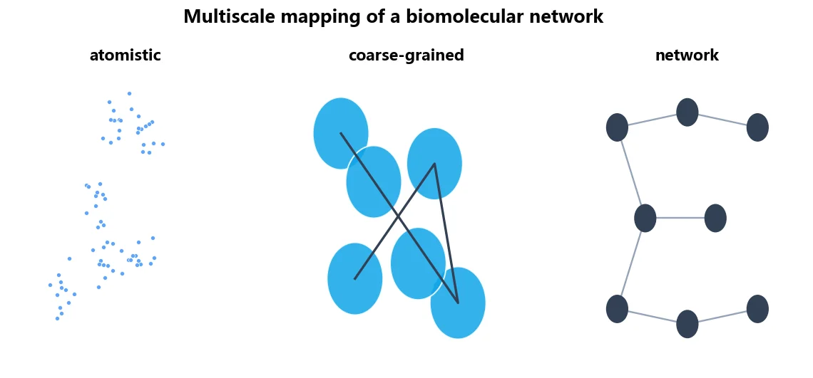
A useful mapping starts from a clear statement of the target quantity. If the goal is to reproduce the elastic modulus of a network, the mapping can discard most intramolecular chemistry and preserve only the connectivity, excluded volume, and crosslink density. If the goal is to distinguish crystalline and amorphous regions, the mapping must retain enough bead specificity to encode both states and their interfaces.
Several common choices dominate the biomaterials literature. MARTINI-style models map several heavy atoms to one bead and separate the bead types by polarity and hydrogen-bonding tendency; they are convenient when lipid, protein, and water compartments must share a single force field. Structure-based or Go-like models place one bead per monomer or residue and encode only the native contacts, which makes them extremely efficient for folding and large-scale rearrangement but too restrictive for studying denaturation or solvent-driven swelling. Network models often go further and represent an entire fiber segment as a single elastic element, which is appropriate for topology and failure statistics but not for local chemistry.
The table below summarizes how the same material can be mapped at progressively coarser levels.
| Mapping level | Representative unit | What it preserves | What it usually loses |
|---|---|---|---|
| --- | --- | --- | --- |
| Atomistic | each atom | charges, bonds, detailed conformations | accessible time and length |
| MARTINI-like | several heavy atoms per bead | polarity and hydrogen-bond character | torsional chemistry details |
| Residue/monomer | one bead per residue or monomer | chain connectivity and native contacts | side-chain packing |
| Network | one site per Kuhn segment | topology and crosslink density | local structure entirely |
Interaction Potentials and Their Limits
The functional form of a coarse-grained potential matters less than the recognition that every coarse-grained force field is a statistical construct. The soft repulsion, bond springs, angular potentials, and pair attractions are not measurements of individual covalent or hydrogen bonds; they are effective interactions chosen so that an ensemble average at the coarse-grained resolution reproduces a chosen reference. This means a parameter set is never universally transferable. A MARTINI parameterization built for membrane bilayers will not automatically describe a crystalline silk-beta-sheet interface without recalibration.
Practical simulations therefore combine bonded and nonbonded terms with care. Bonds and angles can often be fit directly from atomistic distributions using Boltzmann inversion. Nonbonded terms are harder; popular choices include Lennard-Jones repulsion plus screened electrostatic interactions for charged groups, but the screening length and the assignment of partial charges are among the most sensitive choices in the model. Whenever possible, run a small atomistic simulation of the same chemistry first, project the observed pair distributions onto the bead centers, and use those distributions as the target for the coarse-grained potential.
It helps to keep one mental image in place when building these potentials: a bead is not a molecule, it is a crowd of molecules represented by a single moving point, and the interaction between two beads is not a bond between two specific atoms, it is the average push and pull of two crowds that can never be resolved inside the model. If a street has thousands of pedestrians, the average spacing between strangers follows rules that no individual stride embodies; an effective potential captures exactly that statistical, crowd-level rule, which is also why it only works at the temperature, density, and composition where the crowd behavior was measured.
A concrete water example makes the limitation tangible. A popular four-to-one water bead reproduces the density and surface tension of liquid water at room temperature remarkably well, because those are cooperative properties that survive losing the hydrogen-bond directions. It is much less trustworthy near an interface where water molecules line up in an orientational pattern, because that orientation was averaged away in building the bead. The same logic appears in polymer networks: coarse-grained bonds between chain beads can preserve chain stiffness and density, but a single isotropic bead cannot know whether a neighboring residue is polar, charged, or hydrophobic unless that chemical character is explicitly reintroduced through bead type or an angular potential.
Building the force field can follow a bottom-up, top-down, or mixed route, and each has a different relationship to the truth. Bottom-up methods take atomistic simulation as the reference: run a short all-atom trajectory of the same chemistry, project the pair distance distributions, bond and angle distributions onto the bead centers, and invert those distributions with an iteration such as Boltzmann inversion or iterative Boltzmann inversion to obtain effective potentials. The resulting model is faithful to the reference but only at the state point where the reference was generated; change temperature, density, or composition too much and the potentials have to be rebuilt.
Top-down methods instead parameterize against macroscopic experiments, choosing the stiffness of springs, the nonbonded repulsion, and the crosslink density so that the model reproduces a modulus, a mesh size, or a transition temperature. This route does not inherit any short-range chemistry, but it is often the fastest way to make a model that is useful for engineering, provided the target experiment is not also the only validation. Mixed or hybrid approaches are increasingly common: start top-down to match the global mechanics, then locally refine the potentials bottom-up from atomistic distributions in the regions where chemistry matters. In every case, the workflow should be scripted so that the reference distributions, the fitted potentials, and the verification observables are saved alongside the final trajectory; a coarse-grained paper without this provenance is nearly impossible to audit.
Simulation Setup and Equilibration
Coarse-grained simulations are faster than their atomistic parents, but they are still large enough to require a disciplined setup. Build the system with a periodic box larger than twice the longest relevant correlation length, otherwise the network will feel artificial images of itself. Choose bead masses that keep stable integration with a larger timestep, but do not invent smaller masses merely to run faster; the mass distribution changes how the system distributes kinetic energy between stiff and soft degrees of freedom.
Equilibration must be treated as a physical question rather than a formality. Begin with a steep energy minimization of the prepared coordinates, then run gradually heated short simulations with position restraints on the network junctions, and finally remove the restraints only after the solvent-like beads have visibly randomized. A coarse-grained network equilibrates when several independent observables—total energy, box dimensions, chain end-to-end distance, and radial distribution functions—reach stationary fluctuations that do not drift over at least as long as the subsequent production run.
Validation should produce a single, transparent comparison rather than a collection of impressions. The cleanest workflow compares three numbers side by side: the atomistic target, the experimental target, and the coarse-grained prediction. For a fiber network, these three numbers might be the low-strain modulus, the onset of strain stiffening, and the alignment order parameter at a fixed extension. If the coarse-grained model reproduces the atomistic target it was fitted to, that is necessary but not sufficient; the decisive test is whether it also lands near the experimental target that was never used in the fit. Where the three numbers agree, the mapping is doing the job it was designed for. Where they disagree, the disagreement is usually more informative than the agreement, because it localizes which physical process the coarse-graining removed.
Uncertainty also belongs in the comparison. Coarse-grained trajectories look smooth, but the observables built from them still have statistical and sampling error, and a modulus estimated from three independent replicas may have a broader confidence interval than the figure suggests. Standard block averaging, replica-to-replica variation, and a statement of the simulation box and production length are the minimum needed to decide whether a two-percent difference between model and experiment is real or noise. A published agreement without error bars and without the validation observables named in advance is not a validated model; it is a post hoc match that may have been selected from a larger family of failed comparisons.
Validation Before Prediction
Validation is what separates a coarse-grained model from a well-parameterized animation. The minimum standard is to reproduce the atomistic reference that generated the force field: pair distributions, local density, and the probability distributions of bonds and angles. That alone, however, is an in-sample check and should never be advertised as predictive ability. The second, more decisive test is to compute a set of observables that were not used during parameterization—the elastic modulus, chain alignment under extension, network connectivity statistics, or a temperature-dependent structural transition—and compare them to an independent simulation or experiment.
Where experiments exist, compare to observables that are robust to experimental and simulation uncertainty at the same time. Modulus and alignment order parameters are usually safer comparison targets than absolute free energies or rare-event rates. Where experiments do not exist, the model's job is to frame a falsifiable prediction whose outcome, if measured later, would visibly support or reject the coarse-grained mapping.
A useful discipline borrowed from machine learning is to call parameterization "training" and validation "testing," and then to refuse any result that was used in both stages. The pair distribution, density, and bonded distributions that produced a force field answer the in-sample question "did the fitting procedure converge to its target." They do not answer the harder question "does this model describe the material." The hard answer can only come from held-out observables such as the elastic stiffness, the anisotropy of alignment under tension, or a phase-transition temperature that was not among the fitting targets.
Where possible, choose validation quantities that are large-scale and thereby smooth away the molecular noise that coarse-grained models are allowed to get wrong. A modulus or an order parameter is generally a better bridge to experiment than an absolute free energy, because the latter is sensitive to every short-range detail that coarse-graining deliberately discards. A model that gets the modulus and the alignment right while admitting that short-range packing is approximate is often more useful for biomaterial design than a model that reproduces a local pair correlation perfectly and says nothing falsifiable about mechanics.
Understanding the practical workflow makes the abstract discussion of potentials concrete. A representative coarse-grained study begins by selecting an engine and integrator. GROMACS and LAMMPS are the two most common open engines, and both are comfortable with bead-based systems once the topology is written in their formats; a timestep of 10 to 40 femtoseconds is typical for medium-grained models, one or two orders of magnitude larger than an atomistic engine would tolerate, which is where most of the speed gain appears. The thermostat must be chosen for the phenomenon under study. A Langevin or dissipative particle dynamics thermostat adds a controlled random and friction force that also acts as an implicit solvent, which is convenient for chains in solution but damps inertial modes; a Nosé-Hoover thermostat preserves deterministic dynamics better and is preferable when energy transport or stress fluctuation matters. Stating the integrator, thermostat, and the time constant is as important as stating the force field.
System construction and initial geometry demand their own layer of sanity checks. Overlapping beads at the start of a simulation create enormous forces that can tear a network apart before equilibration begins, so coordinates should be generated with a packing or backmapping algorithm that avoids hard overlaps, followed by a steep energy minimization. Periodic boundary conditions must be checked against the slowest structural mode: the box should be several times larger than the largest chain or pore the analysis will measure. A quick visual or histogram check that the density, the pore-size distribution, and the fraction of native contacts are stable during the first part of the run catches most setup errors before they become publications.
The difference between a trajectory that proves something and a trajectory that merely illustrates something is the discipline of pre-registered observables. Decide before running the production simulations which quantities will be computed and with which estimators, then log them at fixed intervals across the run. Total energy, temperature, pressure, box dimensions, chain end-to-end distance, and specific order parameters are reliable sentinels. If any of these drifts in the second half of a supposedly equilibrated production run, the gentle conclusion is more equilibration and the honest conclusion is that the system is changing state. Reading trajectories directly, rather than only the final averages, is what turns a smooth-looking figure into a statement that can survive contact with a skeptical reviewer.
Common Failure Modes and Reporting Standards
The cheapest signature that a coarse-grained model has not been validated is a figure of merit computed in the regime where the model was fitted. More subtle failures include a collapsed chain that never relaxes because the cutoff radius is too short, a box that is too small for the slowest mode, and a hydrogen-bond representation so soft that a supposedly crystalline domain melts during ordinary equilibration. Each of these is detectable by monitoring the raw trajectories and the energy conservation, not only the final averages.
A defensible simulation report therefore names the mapping, the reference used to build the potential, the cutoff and electrostatics treatment, the box dimensions, the thermostat and integrator, the equilibration duration, and the specific validation observables. Without these details, a coarse-grained result is difficult to reproduce and even more difficult to trust.
A thirty-minute audit for a coarse-grained study
To make the reporting standards practical, they can be compressed into a thirty-minute audit that any author can run before submission and any reviewer can run while reading. First, can the mapping be reconstructed from the methods? If the number of atoms per bead, the bead types, and the basis for those choices are not stated, the model is not yet reproducible. Second, can the potentials be reconstructed? The functional form of every bonded and nonbonded term, the cutoff, the treatment of electrostatics, and the reference used to fit each term must be recoverable from the paper plus its supporting information. Third, can the simulation protocol be rerun? The box dimensions, number of beads, integrator, timestep, thermostat, equilibration length, and production length should read like a recipe rather than a summary. Fourth, are the validation observables named, and were any of them used in fitting the force field? If the answer to the first clause is no, the validation is impressionistic; if the answer to the second clause is yes, it is circular. Fifth, is uncertainty reported from independent replicas rather than from a single trajectory?
These five questions expose nearly all the failure modes discussed above without needing to run anything. They also expose the asymmetry that matters most: it is easy to make a coarse-grained simulation produce a plausible-looking number, and comparatively hard to make it produce a number whose provenance can be reconstructed. The audit is not gatekeeping; it is the checklist that converts a demonstration into evidence, and evidence is what an engineering or biomaterials audience can actually build on.
References
- Marrink, S. J., Risselada, H. J., Yefimov, S., Tieleman, D. P., and de Vries, A. H. The MARTINI force field: coarse grained model for biomolecular simulations. J. Phys. Chem. B, 2007.
- Kmiecik, S., Gront, D., Kolinski, M., Wieteska, L., Dawid, A. E., and Kolinski, A. Coarse-grained protein models and their applications. Chem. Rev., 2016.
- Noid, W. G. Perspective: Coarse-grained models for biomolecular systems. J. Chem. Phys., 2013.
- Saunders, M. G., and Voth, G. A. Coarse-graining methods for computational biology. Annu. Rev. Biophys., 2013.