AFM力曲线分析:信号标定与弹性模量拟合
目录
为什么写这个教程
做AFM力谱实验的朋友都知道:仪器导出一堆txt文件,在商业软件里手动处理几个小时。这个教程给你一套完整的Python流程,从读数据到出杨氏模量,不依赖任何商业软件。只用numpy、scipy、matplotlib。
核心分析流程
1. AFM力曲线数据结构
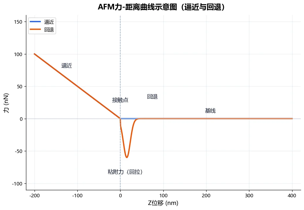
一次典型的AFM力曲线记录的是微悬臂偏转随压电陶瓷移动趋近和远离样品:
| 阶段 | 物理含义 | 提取参数 |
|---|---|---|
| 逼近 | 针尖向样品靠近 | 接触点、样品刚度 |
| 接触 | 针尖压入样品 | 弹性模量 (通过拟合) |
| 回退 | 针尖拉离样品 | 粘附力、解结合事件 |
import numpy as np
import matplotlib.pyplot as plt
from scipy import signal, optimize
2. 加载典型数据
绝大多数AFM仪器导出的是表格数据,常见格式:
- Bruker/Veeco:
.txt,头部以\开头的注释行 - JPK:
.txt或.jpk-force,带元数据头 - Asylum:
.txt或.ibw(可用igorpro包读取) - 通用:
.csv,列为 Z_piezo、Deflection
def load_afm_curve(filepath, skip_rows=0):
    """加载通用AFM力曲线文件"""
    data = np.loadtxt(filepath, skiprows=skip_rows)
    return data[:, 0], data[:, 1]

# 示例:Bruker力曲线
z_piezo, deflection = load_afm_curve("force_curve_001.txt", skip_rows=320)
处理Bruker头部
Bruker NanoScope文件头部长度不固定,下面是自动检测的鲁棒方法:
def load_bruker_curve(filepath):
    """自动检测Bruker头部长度并加载数据"""
    with open(filepath, "r") as f:
        lines = f.readlines()
    skip = 0
    for i, line in enumerate(lines):
        if line.strip().startswith("\\*") or "Ciao" in line:
            skip = i + 1
    data = np.loadtxt(filepath, skiprows=skip)
    return data[:, 0], data[:, 1]
3. 偏转-力转换
微悬臂偏转(单位:伏特)需转换为力(单位:纳牛):
def deflection_to_force(deflection_V, spring_constant, sensitivity_nm_per_V):
    """将偏转从伏特转换为力"""
    deflection_nm = deflection_V * sensitivity_nm_per_V
    force_N = spring_constant * deflection_nm * 1e-9
    return force_N * 1e9  # 转换为纳牛
典型值:软悬臂(如Bruker MLCT)
k = 0.06        # N/m,悬臂弹性常数
sensitivity = 45.0  # nm/V,偏转灵敏度
force = deflection_to_force(deflection, k, sensitivity)
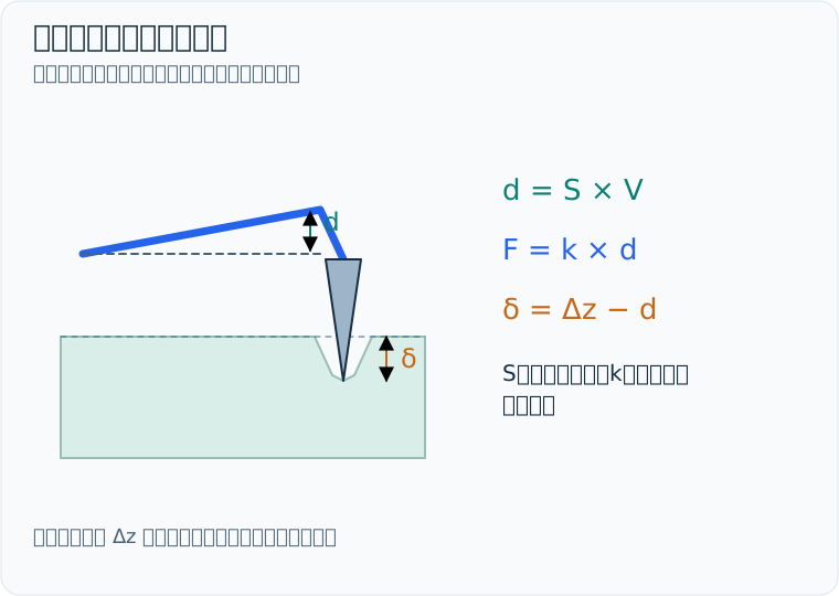
标定后由偏转 d = SV 得到力 F = kd。取压向样品为压电位移正方向并扣除偏移后,压入深度为 δ = Δz − d;几何关系明确了压电位移与样品压入的区别。
4. 基线校正
非接触区的力曲线应该是平坦的(零力),但实际中存在热漂移和激光干涉造成的微小斜率:
def baseline_correct(z_piezo, force, contact_idx):
    """使用接触前区域进行线性基线校正"""
    baseline_region = slice(0, contact_idx)
    coeffs = np.polyfit(
        z_piezo[baseline_region], force[baseline_region], 1
    )
    baseline = np.polyval(coeffs, z_piezo)
    return force - baseline
5. 接触点检测
这是最关键的步骤。稳健方法:找力的导数显著偏离基线噪声的地方。
def find_contact_point(z_piezo, force, window=50, threshold_factor=5):
    """用导数阈值法定位针尖-样品接触点"""
    force_smooth = signal.savgol_filter(
        force, window_length=21, polyorder=3
    )
    dz = np.gradient(z_piezo)
    df = np.gradient(force_smooth)
    derivative = df / dz

    noise_region = slice(0, len(force) // 5)
    noise_std = np.std(derivative[noise_region])
    threshold = threshold_factor * noise_std

    above_threshold = np.abs(derivative) > threshold
    for i in range(len(above_threshold) - window):
        if np.all(above_threshold[i:i + window]):
            return i + window // 2
    raise ValueError("未找到接触点,请检查逼近段")

contact_idx = find_contact_point(z_piezo, force)
contact_z = z_piezo[contact_idx]
print(f"接触点: z = {contact_z:.1f} nm")
6. 粘附力提取
回退曲线上的最小力就是粘附力(拔拉事件):
def extract_adhesion(z_piezo, force, contact_idx):
    """从回退段提取粘附力"""
    retract_region = force[contact_idx:]
    if len(retract_region) == 0:
        return 0.0
    adhesion_idx = np.argmin(retract_region)
    adhesion_force = retract_region[adhesion_idx]
    return adhesion_force if adhesion_force < 0 else 0.0
7. Hertz模型拟合杨氏模量
球形压头在弹性半空间上的Hertz模型:
F = (4/3) E* sqrt(R) delta^(3/2)
其中 E* = E / (1 - nu^2)。
拟合函数接收逼近段,z 采用 nm、力采用 nN,返回的 E 为 Pa。应显式传入实测弹簧常数(N/m)和针尖半径。默认逼近时 z 减小;若仪器记录相反,使用 +1。拟合压入深度应远小于球形针尖半径,样品厚度应明显大于接触半径 a = sqrt(Rδ)。下方参数与教学曲线一致。
def hertz_sphere(indentation, E_star, R):
    """SI units: indentation and R in m, E_star in Pa, force in N."""
    return (4/3) * E_star * np.sqrt(R) * np.power(
        np.maximum(indentation, 0), 1.5
    )

def fit_youngs_modulus(z_piezo, force, contact_idx,
                        tip_radius_nm=5000.0, poisson=0.5,
                        fit_range_nm=200.0, spring_constant=0.06,
                        approach_direction=-1):
    """拟合逼近段:z 用 nm,力用 nN;返回 Pa 单位的模量与拟合误差。"""
    if spring_constant <= 0 or tip_radius_nm <= 0:
        raise ValueError("Spring constant and tip radius must be positive")
    if approach_direction not in (-1, 1):
        raise ValueError("approach_direction must be -1 or +1")
    z_nm = np.asarray(z_piezo, dtype=float)
    force_nN = np.asarray(force, dtype=float)
    contact_force_nN = force_nN - force_nN[contact_idx]
    advance_nm = approach_direction * (z_nm - z_nm[contact_idx])
    deflection_nm = contact_force_nN / spring_constant
    indentation_nm = advance_nm - deflection_nm
    fit_mask = (
        (np.arange(len(z_nm)) >= contact_idx)
        & (indentation_nm > 0) & (indentation_nm < fit_range_nm)
        & (contact_force_nN > 0)
        & np.isfinite(indentation_nm) & np.isfinite(contact_force_nN)
    )
    if np.count_nonzero(fit_mask) < 50:
        return np.nan, np.nan
    indentation_m = indentation_nm[fit_mask] * 1e-9
    radius_m = tip_radius_nm * 1e-9
    force_fit_nN = contact_force_nN[fit_mask]

    def model(delta_m, E_star_Pa):
        return hertz_sphere(delta_m, E_star_Pa, radius_m) * 1e9

    popt, pcov = optimize.curve_fit(
        model, indentation_m, force_fit_nN,
        p0=[1e4], bounds=(1, 1e9)
    )
    E = popt[0] * (1 - poisson**2)
    E_std = np.sqrt(pcov[0, 0]) * (1 - poisson**2)
    return E, E_std
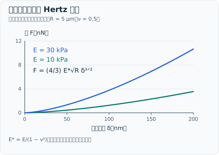
取 R = 5 μm、ν = 0.5、E = 10 或 30 kPa 计算 Hertz 曲线,可比较相同压入深度下模量对力的影响。模型采用刚性球形压头、均匀弹性半空间与可忽略黏附的假设,图中为解析教学曲线。
批量处理与进阶主题
8. 批量处理
一次典型实验通常有几十条力曲线:
import glob
from pathlib import Path

def batch_process_curves(data_dir, k=0.06, sensitivity=45.0, approach_direction=-1):
    """批量处理AFM力曲线,提取力学性能"""
    results = []
    for filepath in sorted(glob.glob(f"{data_dir}/*.txt")):
        try:
            z, deflection = load_afm_curve(filepath, skip_rows=320)
            force = deflection_to_force(deflection, k, sensitivity)
            turn_idx = int(np.argmax(approach_direction * z))
            z_approach = z[:turn_idx + 1]
            cidx = find_contact_point(z_approach, force[:turn_idx + 1])
            force_corr = baseline_correct(z, force, cidx)
            adhesion = (extract_adhesion(z, force_corr, turn_idx)
                        if turn_idx + 1 < len(z) else np.nan)
            E, E_std = fit_youngs_modulus(
                z_approach, force_corr[:turn_idx + 1], cidx,
                tip_radius_nm=5000.0, poisson=0.5,
                spring_constant=k, approach_direction=approach_direction
            )
            results.append({
                "file": Path(filepath).name,
                "contact_z_nm": z[cidx],
                "adhesion_nN": adhesion,
                "youngs_modulus_Pa": E,
            })
        except Exception as e:
            print(f"失败: {Path(filepath).name}: {e}")
    return results

# 使用示例
# results = batch_process_curves("./afm_data/")
# import pandas as pd
# df = pd.DataFrame(results)
# df.to_csv("mechanical_properties.csv", index=False)
9. 常见坑
| 问题 | 可能原因 | 解决方法 |
|---|---|---|
| 接触点太早 | 基线噪声大 | 增大 threshold_factor |
| 负杨氏模量 | 接触点方向反了 | 检查z_piezo符号约定 |
| 基底效应 | 压入深度过大 | fit_range_nm < 样品厚度10% |
| 零粘附 | 回退段未记录 | AFM方法中启用回退 |
| 结果离散 | 样品不均或针尖污染 | 逐条检查再批量拟合 |
10. 替代模型
Hertz假设线弹性。对粘弹性生物材料,考虑:
- JKR模型(Johnson-Kendall-Roberts):包含接触力学中的粘附
- Ting模型:适用于粘弹性松弛
- Sneddon模型:锥形压头(半角alpha)
def sneddon_cone(indentation, E_star, alpha_deg=18):
    """Sneddon锥形压头"""
    alpha = np.radians(alpha_deg)
    return (2 / np.pi) * E_star * np.tan(alpha) * np.power(indentation, 2)
参考资料
- Cappella, B. & Dietler, G. (1999). Force-distance curves by atomic force microscopy. Surface Science Reports, 34(1-3), 1-104.
- Hertz, H. (1882). On the contact of elastic solids. J. Reine Angew. Math., 92, 156-171.
- Sneddon, I.N. (1965). The relation between load and penetration. Int. J. Eng. Sci., 3(1), 47-57.
- JPK Instruments Application Note: A Practical Guide to AFM Force Spectroscopy and Data Analysis.
- Cappella, B. & Dietler, G. (1999). Force-distance curves by AFM. Surface Science Reports, 34(1-3), 1-104.
- Hermanowicz, P. et al. (2014). AtomicJ: An open source software for analysis of force curves. Review of Scientific Instruments, 85(6), 063703.
讨论:AFM力谱学在生物材料定量分析中的进展
AFM力谱学已经从接触模式下的简单力曲线记录发展为一个成熟的定量纳米力学分析平台。峰值力轻敲模式代表了技术上的重要进步——它在每个像素点记录完整的力曲线,同时保持了与传统轻敲模式相当的成像速度。这意味着你可以在一张图像中同时获得形貌信息和定量力学信息,大大提高了实验效率。
粘附力映射在生物材料表征中具有特殊价值。丝素蛋白、胶原蛋白和细胞外基质等材料表现出复杂的表面化学特性,粘附力分布可以揭示表面功能化、蛋白质吸附和交联密度的空间变化。将粘附力映射与形貌像叠加,可以直观地将表面化学性质与结构特征联系起来。
数据处理的标准化和自动化是当前的研究热点。不同的基线校正方法、接触点确定算法和拟合模型可能导致同一组数据得到显著不同的模量值。开源数据处理工具如AtomicJ和PyJibe正在推动AFM数据分析的标准化。建立社区共识的数据处理流程对于提高研究的可复现性和可比性至关重要。